B\(_0\) Inhomogeneity Correction

Here, we are going to have a look at how to correct for B\(_0\) inhomogeneity in MRI data.

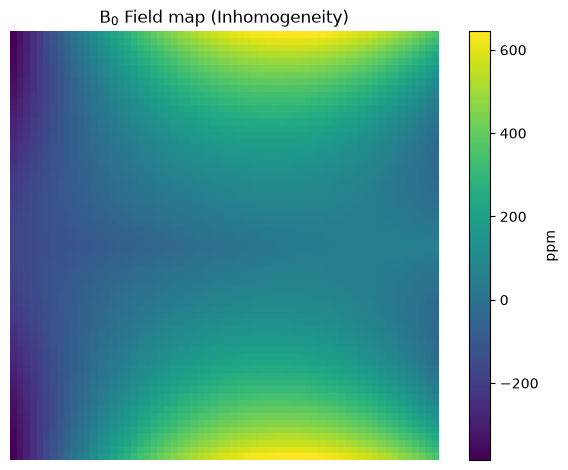
Generate a field map and a simple phantom

We use an ellipse phantom and a random field map to simulate B\(_0\) inhomogeneity.

import mrpro
import torch

matrix = mrpro.data.SpatialDimension(z=1, y=64, x=64)
img = mrpro.phantoms.EllipsePhantom().image_space(matrix)
b0_map = mrpro.phantoms.random_b0map(matrix, fov=matrix * 1e-3, l_max=3, sigma_ppm=1000, seed=1)

Let’s have a look at the field map

import matplotlib.pyplot as plt

plt.imshow(b0_map.squeeze())
plt.colorbar(label='ppm')
plt.title('B$_0$ Field map (Inhomogeneity)')
plt.axis('off')
plt.tight_layout()
plt.show()

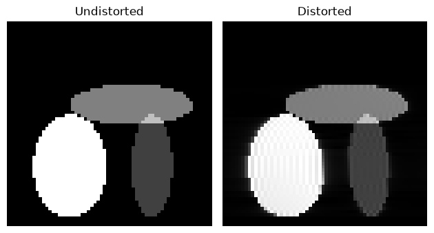
Simulate distorted k-space data

We simulate distorted k-space data by applying the B\(_0\)-informed Fourier operator to the phantom.

ro_bandwidth = 20e3
t_ro = torch.arange(matrix.x) / ro_bandwidth

fourier_op = mrpro.operators.FastFourierOp(dim=(-1, -2))
b0_fourier_op = mrpro.operators.ConjugatePhaseFourierOp(fourier_op=fourier_op, b0_map=b0_map, readout_times=t_ro)
(distorted_k,) = b0_fourier_op(img)

A simple inverse Fourier transform of the distorted k-space data gives us the distorted image.

(distorted_img,) = fourier_op.H(distorted_k)


vmin, vmax = img.abs().aminmax()
fig, ax = plt.subplots(1, 2)
ax[0].imshow(img.abs().squeeze(), cmap='gray', vmin=vmin, vmax=vmax)
ax[0].set_title('Undistorted')
ax[1].imshow(distorted_img.abs().squeeze(), cmap='gray', vmin=vmin, vmax=vmax)
ax[1].set_title('Distorted')
ax[0].axis('off')
ax[1].axis('off')
plt.tight_layout()

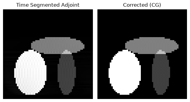
Correct for B0 inhomogeneity

We can use a faster approximation of the B0-informed Fourier operator, namely the Time-Segmented operator. The adjoint already fixes geometric distortions, using conjugate gradient (CG) we can actually invert the operator and also fix intensity inhomogeneities. This is necessry, as F^H F != I for B0-informed Fourier operators!

ts_fourier_op = mrpro.operators.TimeSegmentedFourierOp(fourier_op=fourier_op, b0_map=b0_map, readout_times=t_ro)

(b0_informed_img,) = ts_fourier_op.H(distorted_k)
(corrected_img,) = mrpro.algorithms.optimizers.cg(ts_fourier_op.gram, b0_informed_img)


fig, ax = plt.subplots(1, 2)
ax[0].imshow(b0_informed_img.abs().squeeze(), cmap='gray', vmin=vmin, vmax=vmax)
ax[0].set_title('Time Segmented Adjoint')
ax[1].imshow(corrected_img.abs().squeeze(), cmap='gray', vmin=vmin, vmax=vmax)
ax[1].set_title('Corrected (CG)')
ax[0].axis('off')
ax[1].axis('off')
plt.tight_layout()

Summary

We have explored how to use the B0-informed Fourier operators to generate distorted k-space data and and how to correct for B0 inhomogeneity in the reconstruction.