Motion-corrected image reconstruction

Physiological motion (e.g. due to breathing or the beating of the heart) is a common challenge for MRI. Motion during the data acquisition can lead to motion artifacts in the reconstructed image. Mathematically speaking, the motion occurring during data acquisition can be described by linear operators \(M_m\) for each motion state \(m\):

\( y = [A_m M_m x_{\mathrm{true}}]_m + n, \)

where \(y\) is the acquired k-space data, \(A_m\) is the acquisition operator describing which data was acquired in motion state \(m\) and \(n\) describes complex Gaussian noise.

There are different approaches of how to minimize the impact of motion. The simplest approach is to acquire data only in a single motion state by e.g. asking the subject to hold their breath or synchronize the acquisition with the heart beat. This reduces the above problem to

\( y = A x_{\mathrm{true}} + n, \)

but this is not always possible and can also lead to long acquisition times.

A more efficient approach is to acquire data in different motion states, estimate \(M_m\) and solve the above problem. This is often referred to motion-corrected image reconstruction (MCIR). For some examples have a look at Kolbitsch et al., JNM 2017, Ippoliti et al., MRM 2019 or Mayer et al., JNM 2021

Here we will show how to do a MCIR of a free-breathing acquisition of the thorax following these steps:

1. Estimate a respiratory self-navigator from the acquired k-space data

2. Use the self-navigator to separate the data into different breathing states

3. Reconstruct dynamic images of different breathing states

4. Estimate non-rigid motion fields from the dynamic images

5. Use the motion fields to obtain a motion-corrected image

Data acquisition

The data was acquired with a Golden Radial Phase Encoding (GRPE) sampling scheme [Prieto et al., MRM 2010]. This sampling scheme combines a Cartesian readout with radial phase encoding in the 2D ky-kz plane. The central k-space line (i.e. 1D projection of the object along the foot-head direction) is acquired repeatedly and can be used as a respiratory self-navigator. This sequence was implemented in pulseq and also available as a seq-file. The FOV of the scan was 288 x 288 x 288 \(mm^3\) with an isotropic resolution of 1.9 mm.

Note

To keep reconstruction times short, we used a short acquisition of less than one minute. We also only split the data into 4 motion states with rather large overlap (sliding-window) between motion states. For reliable motion correction at least 6 motion states should be used.

Show import and download details Hide code cell content

# Download raw data and pre-calculated motion fields from zenodo into a temporary directory
import os
import tempfile
from collections.abc import Sequence
from pathlib import Path

import mrpro
import numpy as np
import torch
import zenodo_get
from einops import rearrange

tmp = tempfile.TemporaryDirectory()  # RAII, automatically cleaned up
data_folder = Path(tmp.name)
zenodo_get.download(
    record='15849308', retry_attempts=5, output_dir=data_folder, access_token=os.environ.get('ZENODO_TOKEN')
)

Motion-corrupted image reconstruction

As a first step we will reconstruct the image using all the acquired data which will lead to an image corrupted by respiratory motion.

Note

To reduce the file size we have already applied coil compression reducing the 21 physical coils to 6 compressed coils. We also removed the readout oversampling.

kdata = mrpro.data.KData.from_file(
    data_folder / 'grpe_t1_free_breathing.mrd',
    trajectory=mrpro.data.traj_calculators.KTrajectoryRpe(angle=torch.pi * 0.618034),
)

# Calculate coil maps
csm_maps = mrpro.data.CsmData.from_kdata_inati(kdata, smoothing_width=3, downsampled_size=64)

#  SENSE reconstruction
iterative_sense = mrpro.algorithms.reconstruction.IterativeSENSEReconstruction(kdata, csm=csm_maps)
img = iterative_sense(kdata)

Show plotting details Hide code cell content

import matplotlib.pyplot as plt


def show_views(*images: torch.Tensor, ylabels: Sequence[str] | None = None) -> None:
    """Plot coronal, transversal and sagittal view."""
    if ylabels is not None and len(ylabels) != len(images):
        raise ValueError(f'Expected {len(images)} ylabels, got {len(ylabels)}')
    _, axes = plt.subplots(len(images), 3, squeeze=False, figsize=(12, 4 * len(images)))
    for idx, (image, ylabel) in enumerate(zip(images, ylabels or [''] * len(images), strict=True)):
        image = (image / image.quantile(0.98)).squeeze()
        image_views = [image[:, 61, :], torch.fliplr(image[:, :, 63]), image[54, :, :]]

        for vdx, (view, title) in enumerate(zip(image_views, ['Coronal', 'Transversal', 'Sagittal'], strict=True)):
            axes[idx, vdx].imshow(torch.rot90(view, -1), vmin=0, vmax=1.0 if idx == 1 else 0.8, cmap='grey')
            if idx == 0:
                axes[idx, vdx].set_title(title, fontsize=18)
            axes[idx, vdx].set_xticks([])
            axes[idx, vdx].set_yticks([])
        axes[idx, 0].set_ylabel(ylabel, fontsize=18)
    plt.show()

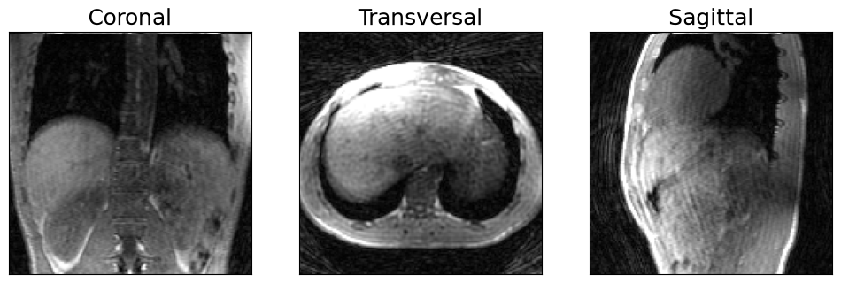
# Visualize anatomical views of 3D image
show_views(img.rss())

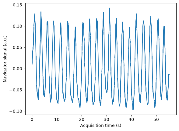
1. Respiratory self-navigator

We are going to obtain a self-navigator from the k-space center line ky = kz = 0 following these steps:

• Get all readout lines for ky = kz = 0

• Apply a 1D FFT along the readout to get the projection of the object

• Carry out SVD over all readout points and all coils to get the main signal components

• Select the SVD component the largest frequency contribution between 0.2 and 0.5 Hz (realistic breathing frequency)

Show self-navigator calculation Hide code cell content

def get_respiratory_self_navigator_from_grpe(
    kdata: mrpro.data.KData, respiratory_frequency_range: tuple[float, float] = (0.2, 0.5)
) -> torch.Tensor:
    """Get respiratory self-navigator from GRPE data set."""
    # Get all readout lines for ky = kz = 0
    kdata_navigator = kdata[(kdata.traj.ky == 0) & (kdata.traj.kz == 0)]

    # Apply a 1D FFT along the readout to get the projection of the object
    fft_op_1d = mrpro.operators.FastFourierOp(dim=(-1,))
    navigator_data = fft_op_1d(kdata_navigator.data)[0].squeeze().abs()

    # Carry out SVD over all readout points and all coils to get the main signal components
    navigator_data = rearrange(navigator_data, 'coil k1k2 k0 -> k1k2 (coil k0)')
    svd_navigator_data, _, _ = torch.linalg.svd(navigator_data - navigator_data.mean(dim=0, keepdim=True))

    # Select the SVD component the largest frequency contribution closest to the expected respiratory frequency
    dt = kdata_navigator.header.acq_info.acquisition_time_stamp.squeeze().diff(dim=0).mean()
    fft_svd_navigator_data = torch.fft.fft(svd_navigator_data, dim=0).abs()
    f_hz = torch.fft.fftfreq(len(svd_navigator_data), dt)
    fft_svd_navigator_data_in_resp_window = fft_svd_navigator_data[
        (f_hz >= respiratory_frequency_range[0]) & (f_hz <= respiratory_frequency_range[1])
    ]
    respiratory_navigator = svd_navigator_data[:, fft_svd_navigator_data_in_resp_window.amax(dim=0).argmax()]

    # Interpolate navigator from k-space center ky=kz=0 to all phase encoding points
    return mrpro.utils.interp(
        kdata.header.acq_info.acquisition_time_stamp.squeeze(),
        kdata_navigator.header.acq_info.acquisition_time_stamp.squeeze(),
        respiratory_navigator,
    )

# To separate all phase encoding points into different motion states we combine ky and kz points along k1 first
kdata = kdata.rearrange('... k2 k1 k0 -> ... 1 (k2 k1) k0')

respiratory_navigator = get_respiratory_self_navigator_from_grpe(kdata)

plt.figure()
acquisition_time = kdata.header.acq_info.acquisition_time_stamp.squeeze()
plt.plot(acquisition_time - acquisition_time.min(), respiratory_navigator)
plt.xlabel('Acquisition time (s)')
plt.ylabel('Navigator signal (a.u.)')

Text(0, 0.5, 'Navigator signal (a.u.)')

2. Split data into different breathing states

The self-navigator is used to split the data into different motion phases. We use a sliding window approach to ensure we have got enough data in each motion state.

# With an overlap of 50% and 4 motion states, 40% of data are in each motion state.
n_points_per_motion_state = int(kdata.shape[-2] * 0.4)
navigator_idx = respiratory_navigator.argsort()
navigator_idx = navigator_idx.unfold(0, n_points_per_motion_state, n_points_per_motion_state // 2)
kdata_resp_resolved = kdata[..., navigator_idx, :]

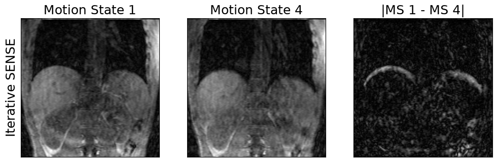
3. Reconstruct dynamic images of different breathing states

recon_resp_resolved = mrpro.algorithms.reconstruction.IterativeSENSEReconstruction(kdata_resp_resolved, csm=csm_maps)
img_resp_resolved = recon_resp_resolved(kdata_resp_resolved)

Show plotting details Hide code cell content

def show_motion_states(image: torch.Tensor, ylabel: str | None = None, slice_idx: int = 61, vmax: float = 0.3) -> None:
    """Plot first and last motion state and difference image."""
    _, axes = plt.subplots(1, 3, squeeze=False, figsize=(12, 16))
    [a.set_xticks([]) for a in axes.flatten()]
    [a.set_yticks([]) for a in axes.flatten()]
    image = (image / image.max()).squeeze()
    axes[0, 0].imshow(torch.rot90(image[0, :, slice_idx, :], -1), vmin=0, vmax=vmax, cmap='grey')
    axes[0, 0].set_title('Motion State 1', fontsize=18)
    axes[0, 0].set_ylabel(ylabel, fontsize=18)
    axes[0, 1].imshow(torch.rot90(image[-1, :, slice_idx, :], -1), vmin=0, vmax=vmax, cmap='grey')
    axes[0, 1].set_title(f'Motion State {image.shape[0]}', fontsize=18)
    axes[0, 2].imshow(
        torch.rot90(image[0, :, slice_idx, :] - image[-1, :, slice_idx, :], -1).abs(), vmin=0, vmax=0.2, cmap='grey'
    )
    axes[0, 2].set_title(f'|MS 1 - MS {image.shape[0]}|', fontsize=18)
    plt.show()

show_motion_states(img_resp_resolved.rss(), ylabel='Iterative SENSE')

4. Estimate the motion fields from the dynamic images

The motion fields can be estimated with an image registration package such as mirtk. Here we registered each of the dynamic respiratory phases to the first motion state using the free-form deformation (FFD) registration approach with a control point spacing of 9. Normalized mutual information was used as a similarity metric and a LogJac penalty weight of 0.001 was applied.

To improve the motion estimation, we used a TV-regularized image reconstruction to obtain the dynamic images. Have a look at TotalVariationRegularizedReconstruction to find out more.

We load the displacement fields and create a motion operator:

mf = torch.as_tensor(np.load(data_folder / 'grpe_t1_free_breathing_displacement_fields.npy'), dtype=torch.float32)
motion_op = mrpro.operators.GridSamplingOp.from_displacement(mf[..., 2], mf[..., 1], mf[..., 0])

5. Use the motion fields to obtain a motion-corrected image

Now we obtain a motion-corrected image \(x\) by minimizing the functional \(F\)

\( F(x) = \sum_m||(A_mx - y_m)||_2^2 \quad\) with \(\quad A_m = F_m M_m C \)

where \(C\) describes the coil-sensitivity maps, \(M_m\) is the motion transformation of motion state \(m\) and \(F_m\) describes the Fourier transform of all of the k-space points obtained in motion state \(m\).

One way to solve this problem with MRpro is to use the respiratory-resolved k-space data from above. Because we used a sliding window approach to split the data into different motion states, this is computationally a bit more demanding than it needs to be but it also doesn’t hurt.

# Create acquisition operator
fourier_op = recon_resp_resolved.fourier_op
csm_op = mrpro.operators.SensitivityOp(csm_maps)
averaging_op = mrpro.operators.AveragingOp(dim=0)
acquisition_operator = fourier_op @ motion_op @ csm_op @ averaging_op.H
operator = acquisition_operator.gram
(right_hand_side,) = acquisition_operator.H(kdata_resp_resolved.data)

# The DCF is used to obtain a good starting point for the CG algorithm.
# This is equivalent to running the CG algorithm with H = A^H DCF A and b = A^H DCF y
# for a single iteration.
if recon_resp_resolved.dcf_op is not None:
    (u,) = (acquisition_operator.H @ recon_resp_resolved.dcf_op)(kdata_resp_resolved.data)
    (v,) = (acquisition_operator.H @ recon_resp_resolved.dcf_op @ acquisition_operator)(u)
    u_flat = u.flatten(start_dim=-3)
    v_flat = v.flatten(start_dim=-3)
    initial_value = (
        mrpro.utils.unsqueeze_right(torch.linalg.vecdot(u_flat, u_flat) / torch.linalg.vecdot(v_flat, u_flat), 3) * u
    )
else:
    initial_value = torch.zeros_like(right_hand_side)

# Minimize the functional by solving operator(x) = right_hand_side with conjugate gradient
(img_mcir,) = mrpro.algorithms.optimizers.cg(
    operator,
    right_hand_side,
    initial_value=initial_value,
    max_iterations=10,
    tolerance=0.0,
)

show_views(img.rss(), img_mcir.abs(), ylabels=('Uncorrected', 'MCIR'))

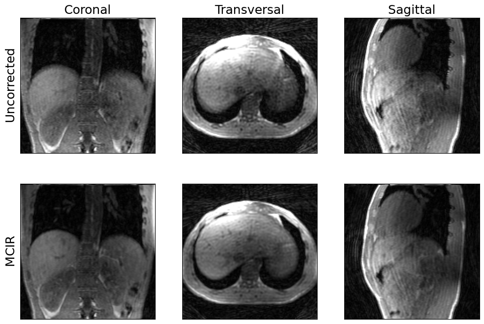
We have used a rather small number of CG iterations here to make sure the reconstruction does not take too long. Increase max_iterations to get an even sharper image.