Cardiac MR Fingerprinting

This notebook provides the image reconstruction and parameter estimation methods required to reconstruct cardiac MR Fingerprinting (cMRF) data.

Overview

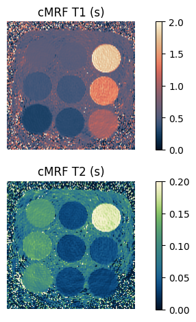
In this notebook, data from a cardiac MR Fingerprinting (cMRF) experiment is reconstructed and \(T_1\) and \(T_2\) maps are estimated. This example uses data from [Schuenke et al., 2024](in submission) of a phantom consisting of 9 tubes. Average \(T_1\) and \(T_2\) are calculated for each tube.

The fingerprinting sequence, as described by Hamilton et al., 2017 and [Schuenke et al., 2024](in submission), consists of three repetitions of the following 5-block structure:

# Block 0          Block 1          Block 2          Block 3          Block 4
# R-peak           R-peak           R-peak           R-peak           R-peak
# |----------------|----------------|----------------|----------------|----------------
# [INV][ACQ]           [ACQ]       [T2-prep][ACQ]      [T2-prep][ACQ]   [T2-prep][ACQ]

where [INV] represents an inversion pulse, [ACQ] an acquisition, and [T2-prep] a T2-preparation pulse.

We carry out dictionary matching to estimate \(T_1\) and \(T_2\) from a series of reconstructed qualitative images using normalized dot product matching between the images and a dictionary of pre-calculated signals. Pixelwise, we find the entry \(d^*\) in the dictionary maximizing \(\left|\frac{d}{\|d\|} \cdot \frac{y}{\|y\|}\right|\) for the reconstructed signal \(y\). The parameters \(x\) generating the matching dictionary entry \(d^*=d(x)\) are then used to estimate the quantitative parameters.

In the following, we are going to:

• Download data from zenodo.

• Reconstruct the qualitative images using a sliding window reconstruction.

• Perform dictionary matching to estimate the quantitative parameters from the qualitative images.

• Visualize and evaluate results.

• Check if the cMRF results match the reference values.

Show download details Hide code cell content

# Download data from zenodo
import tempfile
from pathlib import Path

import zenodo_get

dataset = '15182376'

tmp = tempfile.TemporaryDirectory()  # RAII, automatically cleaned up
data_folder = Path(tmp.name)
zenodo_get.zenodo_get([dataset, '-r', 5, '-o', data_folder])  # r: retries

Reconstruct qualitative images

We first load the data from a downloaded ISMRMRD file.

import mrpro

kdata = mrpro.data.KData.from_file(data_folder / 'cMRF.h5', mrpro.data.traj_calculators.KTrajectoryIsmrmrd())

We want to perform a sliding window reconstruction respecting the block structure of the acquisition. We construct a split index that splits the data into windows of 20 acquisitions with an overlap of 10 acquisitions. Here, we can make use of the indexing functionality of KData to split the data into windows.

import torch

n_acq_per_image = 20
n_overlap = 10
n_acq_per_block = 47
n_blocks = 15

idx_in_block = torch.arange(n_acq_per_block).unfold(0, n_acq_per_image, n_acq_per_image - n_overlap)
split_indices = (n_acq_per_block * torch.arange(n_blocks)[:, None, None] + idx_in_block).flatten(end_dim=1)
kdata_split = kdata[..., split_indices, :]

We can now perform the reconstruction for each window. We first perform an averaged reconstruction over all acquisitions to get a good estimate of the coil sensitivities before performing the windowed reconstruction.

avg_recon = mrpro.algorithms.reconstruction.DirectReconstruction(kdata)
recon = mrpro.algorithms.reconstruction.DirectReconstruction(kdata_split, csm=avg_recon.csm)
img = recon(kdata_split)

Dictionary matching

Next, we calculate the dictionary. First, we set up the CardiacFingerprinting operator and an AveragingOp operator. This AveragingOp mimics the averaging performed by the sliding window reconstruction and applies it to the simulated signals generated by the CardiacFingerprinting model.

model = mrpro.operators.AveragingOp(dim=0, idx=split_indices) @ mrpro.operators.models.CardiacFingerprinting(
    kdata.header.acq_info.acquisition_time_stamp.squeeze(),
    echo_time=0.00155,
    repetition_time=0.01,
    t2_prep_echo_times=(0.03, 0.05, 0.1),
)

Next, we pass this signal model to the DictionaryMatchOp operator to create a dictionary.

dictionary = mrpro.operators.DictionaryMatchOp(model, index_of_scaling_parameter=0)

Next, we choose a suitable range of \(T_1\) and \(T_2\) values for the dictionary. We can keep \(M_0\) constant at 1.0, as dictionary matching is invariant to a scaling factor. By adding these keys to the dictionary, the DictionaryMatchOp operator will use the signal model to calculate the dictionary entries for the given \(M_0\), \(T_1\) and \(T_2\) values.

t1_keys = torch.arange(0.05, 2, 0.01)[:, None]
t2_keys = torch.arange(0.006, 0.2, 0.002)[None, :]
m0_keys = torch.tensor(1.0)
dictionary.append(m0_keys, t1_keys, t2_keys)

Show code cell output Hide code cell output

DictionaryMatchOp(
  (_f): OperatorComposition(
    (_operator1): AveragingOp()
    (_operator2): CardiacFingerprinting(
      (sequence): EPGSequence(
        (0): EPGSequence(
          (0): InversionBlock()
          (1): FispBlock()
        )
        (1): DelayBlock()
        (2): EPGSequence(
          (0): FispBlock()
        )
        (3): DelayBlock()
        (4): EPGSequence(
          (0): T2PrepBlock()
          (1): FispBlock()
        )
        (5): DelayBlock()
        (6): EPGSequence(
          (0): T2PrepBlock()
          (1): FispBlock()
        )
        (7): DelayBlock()
        (8): EPGSequence(
          (0): T2PrepBlock()
          (1): FispBlock()
        )
        (9): DelayBlock()
        (10): EPGSequence(
          (0): InversionBlock()
          (1): FispBlock()
        )
        (11): DelayBlock()
        (12): EPGSequence(
          (0): FispBlock()
        )
        (13): DelayBlock()
        (14): EPGSequence(
          (0): T2PrepBlock()
          (1): FispBlock()
        )
        (15): DelayBlock()
        (16): EPGSequence(
          (0): T2PrepBlock()
          (1): FispBlock()
        )
        (17): DelayBlock()
        (18): EPGSequence(
          (0): T2PrepBlock()
          (1): FispBlock()
        )
        (19): DelayBlock()
        (20): EPGSequence(
          (0): InversionBlock()
          (1): FispBlock()
        )
        (21): DelayBlock()
        (22): EPGSequence(
          (0): FispBlock()
        )
        (23): DelayBlock()
        (24): EPGSequence(
          (0): T2PrepBlock()
          (1): FispBlock()
        )
        (25): DelayBlock()
        (26): EPGSequence(
          (0): T2PrepBlock()
          (1): FispBlock()
        )
        (27): DelayBlock()
        (28): EPGSequence(
          (0): T2PrepBlock()
          (1): FispBlock()
        )
      )
    )
  )
)

We can now perform the dictionary matching by passing the reconstructed image data to the DictionaryMatchOp operator.

m0_match, t1_match, t2_match = dictionary(img.data[:, 0, 0, 0])

Visualize and evaluate results

Great! Now we can visualize and evaluate the results. We can plot the cMRF \(T_1\) and \(T_2\) maps:

Show plotting code Hide code cell content

import matplotlib.pyplot as plt
from cmap import Colormap


def show_image(t1: torch.Tensor, t2: torch.Tensor) -> None:
    """Show the cMRF $T_1$ and $T_2$ maps."""
    cmap_t1 = Colormap('lipari')
    cmap_t2 = Colormap('navia')
    fig, ax = plt.subplots(2, 1)

    im = ax[0].imshow(t1.numpy(force=True), vmin=0, vmax=2, cmap=cmap_t1.to_mpl())
    ax[0].set_title('cMRF T1 (s)')
    ax[0].set_axis_off()
    plt.colorbar(im)

    im = ax[1].imshow(t2.numpy(force=True), vmin=0, vmax=0.2, cmap=cmap_t2.to_mpl())
    ax[1].set_title('cMRF T2 (s)')
    ax[1].set_axis_off()
    plt.colorbar(im)

    plt.tight_layout()
    plt.show()

show_image(t1_match, t2_match)

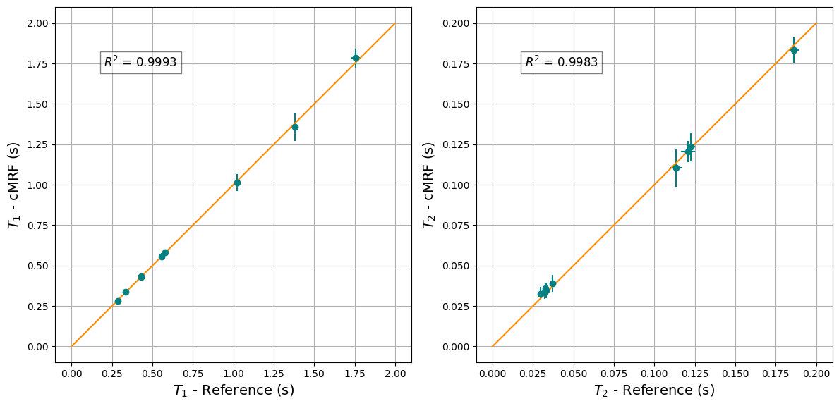
We can also plot the statistics of the cMRF \(T_1\) and \(T_2\) maps and compare them to pre-calculated reference values, obtained from a separate reference scan.

Show statistics helper functions Hide code cell content

import numpy as np


def image_statistics(idat: torch.Tensor) -> tuple[torch.Tensor, torch.Tensor]:
    """Calculate mean value and standard deviation in the ROIs."""
    mask = np.squeeze(np.load(data_folder / 'mask.npy'))
    n_tubes = 9
    mean = torch.stack([torch.mean(idat[mask == idx]) for idx in range(1, n_tubes + 1)])
    std_deviation = torch.stack([torch.std(idat[mask == idx]) for idx in range(1, n_tubes + 1)])
    return mean, std_deviation


def r_squared(true: torch.Tensor, predicted: torch.Tensor) -> float:
    """Calculate the coefficient of determination (R-squared)."""
    total = ((true - true.mean()) ** 2).sum()
    residual = ((true - predicted) ** 2).sum()
    r2 = 1 - residual / total
    return r2.item()

Show plotting code Hide code cell source

# Loading of reference maps and time conversion from ms to s
ref_t1_maps = torch.tensor(np.load(data_folder / 'ref_t1.npy')) / 1000
ref_t2_maps = torch.tensor(np.load(data_folder / 'ref_t2.npy')) / 1000
t1_mean_ref, t1_std_ref = image_statistics(ref_t1_maps)
t2_mean_ref, t2_std_ref = image_statistics(ref_t2_maps)
t1_mean_cmrf, t1_std_cmrf = image_statistics(t1_match)
t2_mean_cmrf, t2_std_cmrf = image_statistics(t2_match)

fig, ax = plt.subplots(1, 2, figsize=(12, 7))
ax[0].errorbar(t1_mean_ref, t1_mean_cmrf, t1_std_cmrf, t1_std_ref, fmt='o', color='teal')
ax[0].plot([0, 2.0], [0, 2.0], color='darkorange')
ax[0].text(
    0.2,
    1.800,
    rf'$R^2$ = {r_squared(t1_mean_ref, t1_mean_cmrf):.4f}',
    fontsize=12,
    verticalalignment='top',
    horizontalalignment='left',
    bbox={'facecolor': 'white', 'alpha': 0.5},
)
ax[0].set_xlabel('$T_1$ - Reference (s)', fontsize=14)
ax[0].set_ylabel('$T_1$ - cMRF (s)', fontsize=14)
ax[0].grid()
ax[0].set_aspect('equal', adjustable='box')

ax[1].errorbar(t2_mean_ref, t2_mean_cmrf, t2_std_cmrf, t2_std_ref, fmt='o', color='teal')
ax[1].plot([0, 0.2], [0, 0.2], color='darkorange')
ax[1].text(
    0.02,
    0.180,
    rf'$R^2$ = {r_squared(t2_mean_ref, t2_mean_cmrf):.4f}',
    fontsize=12,
    verticalalignment='top',
    horizontalalignment='left',
    bbox={'facecolor': 'white', 'alpha': 0.5},
)
ax[1].set_xlabel('$T_2$ - Reference (s)', fontsize=14)
ax[1].set_ylabel('$T_2$ - cMRF (s)', fontsize=14)
ax[1].grid()
ax[1].set_aspect('equal', adjustable='box')

plt.tight_layout()
plt.show()

Show code cell content Hide code cell content

# Assertion verifies if cMRF results match the pre-calculated reference values
torch.testing.assert_close(t1_mean_ref, t1_mean_cmrf, atol=0, rtol=0.15)
torch.testing.assert_close(t2_mean_ref, t2_mean_cmrf, atol=0, rtol=0.15)